The COALA project

The COALA H2020 project is contributing to better agriculture. COALA is implementing tools capable of determining the water and nutrient requirements of crops in space and time. These tools allow farmers to adjust the adequate supply of these resources to optimise yield. These tools are developed using a time series of images acquired by the Sentinel2 satellites of the Copernicus program. These images have excellent characteristics for describing crop development. In terms of temporal resolution, the satellites return to the same place weekly. And in terms of spatial resolution, they have a pixel of 10 m on each side.  These characteristics of Sentinel2 images and their free availability are firsts in Earth Observation applications for agriculture.

Management Zones Maps

Management Zones Maps (MZMs) help us tell farmers their crop nutrient requirements. We derive these MZMs from a time series of Sentinel 2 images. Management Zone Maps capture the spatial distribution of within-field crop growth relative to the field average value.  Ultimately, the MZM aims to capture the differences in within-field soil fertility. These variations can help explain the growth differences between different paddock parts when other factors such as management and meteorology are uniform. The MZM can, among other uses, help you modulate the nutrient amount you apply to the crop in each subzone, according to its differential growth.

Management Zones Map in Australian Paddocks

In the COALA project, a global team of researchers and farmers analysed the use of MZM teams in dryland paddocks of several farms near Horsham and Birchip, Victoria, Au. The below map shows where the farms under analysis are located. These farms belong to Tim, Cam and Rodney.

Surprisingly, in several paddocks of one of Tim´s farm, the MZMs drew a striking granular structure. But for Cam and Rodney’s farms, the pattern was the predicted one.

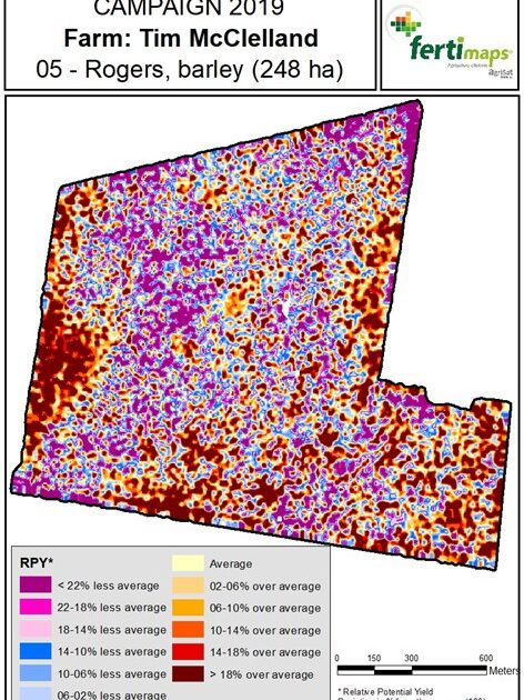
The image above shows the MZM for Tim’s paddock 05-Rogers which exhibits this striking granular structure. The MZM shows the crop canopy’s spatial pattern of variability is similar to other paddocks on this farm. This presence of this granular structure implies that when carrying out a linear transect, it is possible to pass through zones that alternate between higher and lower production in a few tens of metres, which maybe should allow assigning a characteristic length in a cycle. Moreover, the picture suggests a two-dimensional structure without a clear preferential direction. Additionally, this high-frequency spatial pattern seems to overlap another variability on a larger spatial scale, which marks differences between paddock subzones.

A surprise in the Management Zone Maps

The researchers from UCLM & Agrisat who were making these maps were surprised. There was crop cover variability of about several tens of meters of distance from peak to peak, and with a quasi-periodic form, as the granular structure suggests. Really, they had never seen these features before. The usual picture of MZM indicates differences between the subzones of a plot on appropriate spatial scales for agronomic management. This is what also happens in the other farms under study in Australia. In the other farms, the MZM of paddocks exhibits the usual within-field spatial scales without granular structure. You can see that in the image shown above, from a selected typical plot of Cam’s farm, near Horsham.

Therefore, we wanted to know what makes the spatial pattern of variability of Tim’s farm clearly different from Cam and Rodney’s farms.

How MZM picks up the crop growth through Sentinel2 time series

This map is a portion of the first image from Tim’s farm, it shows the variability pattern in detail. The orange to brown coloured areas means an expected higher yield than the field averaged yield value. Blue to purple coloured areas means an expected lower yield than the field averaged yield value. And, the lower part of this image represents the time trajectory of the NDVI value in points indicated by dots. Each point in the graphic is the NDVI value from the Sentinel2 images acquired on the corresponding date.

The NDVI time trajectory for the red dot in the brown area is consistently higher than the time trajectory for the blue dot in the purple area. The NDVI measures the relative photosynthetic activity of the canopy, while the numerical integration of the NDVI curve during the growing cycle links with expected yield. The relative difference in the expected yield for each pixel concerning the average value of the whole paddock is the MZM.

The reason for the variability?

Sharing and discussing these results with Australian colleagues shed light on this phenomenon. The explanation that emerges is that we are in a gilgai area. Therefore, the gilgai soil structure pattern may reflect the crop cover pattern during the growing cycle. Gilgai is a word in Kamilaroi, Wiradhuri and related Aboriginal languages which means waterhole.

MZM mapping gilgai soil structure

A Gilgai soil structure is a micro-relief of the soil characteristic of clayey areas on vertisol soils, with soft mounds and depressions, which form patterns with some degree of symmetry. This micro-relief is due to the shrinking and swelling of soil clays during drying and wetting cycles. These cycles are typical of climates with marked seasonal differences in precipitation and temperature. Likewise, contraction and expansion processes alter the properties of the subsoil and subsurface soil differences are associated with the areas occupied by the mounds and the depressions of the micro-relief.

Gilgai soil structure as the source of high-frequency spatial crop variability

Do the gilgai soil structure characteristics make it possible to explain the spatial pattern observed in the crop cover? We had to consider what the MZM showed, and consider the possible erasure effect that years of agricultural tasks could have had on the pristine structure of the soil.

The MZMs rely on the hypothesis that the variability pattern of the vegetation canopy reflects that of the properties of the soil on which the plant grows. Crop growth is a valuable probe for testing soil fertility. Management Zone Maps derived through Sentinel 2 images pick up the spatial distribution of how crop growth happens.  

If so, in Tim’s paddock, and in other similar ones, the properties of the soil that define its fertility should respond to the same spatial pattern of 2D granular structure observed in the vegetation cover.

Gilgai effects on soil structure

Two effects overlap in the soil structure of the gilgai that can affect crop canopy growing above.

1) In semi-arid areas, micro-relief and cracks prevent surface runoff in abundant rainfalls when the rainy season starts. This process allows efficient water management in depressions when it is scarce.

2) Spatial subsurface soil properties vary on a transect across typical gilgai terrain of the Bland Plain of New South Wales. Gilgais evidently recur fairly regularly on the transect for spectral analysis to reveal a periodicity that exhibits a wavelength of 33.3 m”,

Both surface and subsurface gilgai characteristics exhibit some degree of spatial symmetry. These characteristics are consistent with Tim’s MZM – granular structures and the spatial scale of the canopy crop growth.

So far, no alternative explanation has been found to explain the high-frequency spatial pattern crop canopy cover exhibits.

Although further research and ground truth will be needed, the encouraging results seem to support that the MZM could be a valuable tool for mapping gilgai subsurface soil structures.